Building a Probabilistic Search Engine: Bayesian BM25 and Hybrid Search

Modern search systems face a fundamental challenge: how do you combine lexical matching (exact keyword search) with semantic understanding (meaning-based similarity)? In this article, we explore how we built a probabilistic ranking framework in Cognica Database that transforms traditional BM25 scores into calibrated probabilities, enabling principled fusion of text and vector search results.

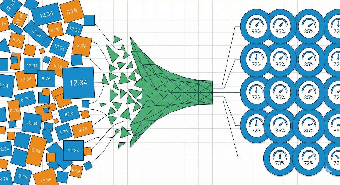
The Problem with Raw BM25 Scores

BM25 (Best Matching 25) is the de facto standard for full-text search ranking. However, its raw scores have a significant limitation: they are unbounded positive real numbers with no absolute meaning.

Consider this search result:

A score of 12.34 tells us nothing about relevance probability. Is this document 90% likely to be relevant? 50%? The score depends on:

• Query length: More terms produce higher scores
• Collection statistics: IDF varies with corpus size
• Document length: Affects the normalization factor

This becomes a critical problem when building hybrid search systems that combine multiple signals.

The Multi-Signal Fusion Challenge

Modern search engines combine multiple ranking signals:

$$\text{FinalScore} = f(\text{text\_relevance}, \text{semantic\_similarity}, \text{freshness}, \text{popularity}, \ldots)$$

When signals have different scales and distributions, naive combination fails:

Naive summation (BM25 dominates):

$$\text{final} = \underbrace{12.34}_{\text{BM25}} + \underbrace{0.85}_{\text{vector}} + \underbrace{0.92}_{\text{fresh}} = 14.11$$

Naive multiplication (still dominated):

$$\text{final} = 12.34 \times 0.85 \times 0.92 = 9.65$$

The unbounded BM25 score overwhelms the normalized signals. We need a principled approach.

Why Not Reciprocal Rank Fusion (RRF)?

A common approach to hybrid search is Reciprocal Rank Fusion (RRF), which combines rankings rather than scores:

$$\text{RRF}(d) = \sum_{r \in R} \frac{1}{k + \text{rank}_r(d)}$$

where $k$ is a smoothing constant (typically 60).

While RRF is simple and robust, it has significant limitations:

1. Discards score magnitude: A document ranked #1 with score 0.99 is treated the same as one ranked #1 with score 0.51. The confidence information is lost.

2. Requires separate retrieval phases: You must retrieve top-k from each system independently, then merge. This prevents joint optimization.

3. Cannot leverage WAND/BMW optimizations: Score-based pruning algorithms like WAND and BMW cannot work with rank-based fusion.

4. Sensitive to k parameter: The smoothing constant $k$ significantly affects results but has no principled way to tune.

5. No probabilistic interpretation: The fused score has no meaningful interpretation; it is just a heuristic combination.

Our probabilistic approach addresses all these limitations by transforming scores into calibrated probabilities that can be combined using probability theory.

Our Solution: Bayesian BM25

We transform BM25 scores into calibrated probabilities using Bayesian inference. The core insight is treating relevance as a latent variable and computing the posterior probability of relevance given the observed BM25 score.

The Mathematical Framework

Starting from Bayes' theorem:

$$P(\text{relevant} \mid s) = \frac{P(s \mid \text{relevant}) \cdot P(\text{relevant})}{P(s)}$$

We model the likelihood using a sigmoid function:

$$P(s \mid \text{relevant}) = \sigma(\alpha \cdot (s - \beta)) = \frac{1}{1 + e^{-\alpha(s - \beta)}}$$

Where:

• $\alpha$: Controls sigmoid steepness (score sensitivity)
• $\beta$: Controls sigmoid midpoint (relevance threshold)

Architecture Overview

Composite Prior Design

Rather than using a flat prior, we incorporate domain knowledge through a composite prior that considers both term frequency and document length:

Term Frequency Prior (weight: 0.7):

$$P_{\text{tf}}(f) = 0.2 + 0.7 \cdot \min\left(1, \frac{f}{10}\right)$$

Documents with higher term frequencies have higher prior probability of relevance.

Field Norm Prior (weight: 0.3):

$$P_{\text{norm}}(n) = 0.3 + 0.6 \cdot \left(1 - \min(1, |n - 0.5| \cdot 2)\right)$$

Documents that are neither too short nor too long have higher prior probability.

The composite prior is:

$$P_{\text{prior}} = 0.7 \cdot P_{\text{tf}} + 0.3 \cdot P_{\text{norm}}$$

Clamped to $[0.1, 0.9]$ to prevent extreme priors from dominating the posterior.

Posterior Probability Computation

The final posterior probability formula derives from Bayes' theorem. Let:

• $L = P(s \mid R) = \sigma(\alpha(s - \beta))$ be the likelihood
• $p = P(R)$ be the prior probability

Then:

$$P(R \mid s) = \frac{L \cdot p}{L \cdot p + (1 - L) \cdot (1 - p)}$$

Implementation:

float compute_posterior_probability_(float score, float prior) const {
  auto likelihood = 1.0f / (1.0f + std::exp(-alpha_ * (score - beta_)));
  auto joint_probability = likelihood * prior;
  auto complement_joint_probability = (1.0f - likelihood) * (1.0f - prior);
  return joint_probability / (joint_probability + complement_joint_probability);
}

This transforms any BM25 score into a probability in $[0, 1]$.

Mathematical Properties:

1. Output Range: Always in $(0, 1)$
2. Monotonicity: Higher BM25 scores yield higher posterior (for $\alpha > 0$)
3. Prior Influence: Prior shifts the decision boundary
4. Calibration: With proper $\alpha, \beta$, outputs approximate true relevance probabilities

Standard BM25 Implementation

Before diving into the Bayesian transformation, let us understand our BM25 implementation.

The Classic BM25 Formula

$$\text{score}(D, Q) = \sum_{t \in Q} \text{IDF}(t) \cdot \frac{f(t, D) \cdot (k_1 + 1)}{f(t, D) + k_1 \cdot \left(1 - b + b \cdot \frac{|D|}{\text{avgdl}}\right)}$$

Where:

• $f(t, D)$: Term frequency of $t$ in document $D$
• $|D|$: Document length (number of terms)
• $\text{avgdl}$: Average document length in collection
• $k_1 = 1.2$: Term frequency saturation parameter
• $b = 0.75$: Document length normalization parameter

Monotonicity-Preserving Implementation

We use a mathematically equivalent but numerically stable form:

$$\text{score} = w - \frac{w}{1 + f \cdot \text{inv\_norm}}$$

where:

$$\text{inv\_norm} = \frac{1}{k_1 \cdot \left((1 - b) + b \cdot \frac{\text{norm}}{\text{avgdl}}\right)}$$

and $w = \text{boost} \cdot \text{IDF}$.

float score(float freq, float norm) const {
  // Monotonicity-preserving rewrite:
  // freq / (freq + norm) = 1 - 1 / (1 + freq * (1 / norm))
  auto inv_norm = 1.f / (k1_ * ((1.f - b_) + (b_ * norm / avg_doc_size_)));
  return weight_ - weight_ / (1.f + freq * inv_norm);
}

This rewriting guarantees:

• Monotonic with term frequency: $f_1 > f_2 \implies \text{score}(f_1, n) \geq \text{score}(f_2, n)$
• Anti-monotonic with document length: $n_1 > n_2 \implies \text{score}(f, n_1) \leq \text{score}(f, n_2)$

IDF Computation

We use the Robertson-Sparck Jones IDF formula:

$$\text{IDF}(t) = \ln\left(\frac{N - \text{df}(t) + 0.5}{\text{df}(t) + 0.5} + 1\right)$$

Where:

• $N$: Total number of documents in the collection
• $\text{df}(t)$: Document frequency (documents containing term $t$)

float compute_idf(int64_t doc_freq, int64_t doc_count) const {
  auto idf = std::log((static_cast<float>(doc_count - doc_freq) + 0.5f)
                          / (static_cast<float>(doc_freq) + 0.5f)
                      + 1);
  return idf;
}

IDF Properties:

• Rare terms (low $\text{df}$) get high IDF
• Common terms (high $\text{df}$) get low IDF
• The $+1$ smoothing ensures IDF is always positive

Document Length Normalization

The normalization factor is applied at scoring time:

$$\text{norm\_factor} = k_1 \cdot \left((1 - b) + b \cdot \frac{|D|}{\text{avgdl}}\right)$$

WAND and BMW Optimization

For efficient top-k retrieval, we implement both WAND (Weak AND) and BMW (Block-Max WAND) algorithms.

WAND Algorithm

WAND skips documents that cannot enter the result set using term-level upper bounds:

Upper Bound Computation:

For BM25, the upper bound is reached as term frequency approaches infinity:

$$\text{upper\_bound} = \lim_{f \to \infty} \text{score}(f, n) = w = \text{boost} \cdot \text{IDF}$$

WAND Pruning Condition:

$$\sum_{i=0}^{\text{pivot}} \text{upper\_bound}_i < \theta \implies \text{skip to next pivot}$$

where $\theta$ is the current $k$-th highest score.

BMW (Block-Max WAND) Algorithm

BMW improves upon WAND by using block-level upper bounds instead of term-level bounds. The posting list is divided into 128-document blocks, and the maximum score within each block is precomputed.

Key Differences from WAND:

Automatic Selection:

bool use_bmw = false;
if (avg_posting_size <= 250) {
  use_bmw = true;  // BMW always wins on small lists
} else if (avg_posting_size <= 1000) {
  use_bmw = true;  // BMW wins 7-17% faster
} else if (avg_posting_size <= 5000) {
  use_bmw = (num_terms <= 3);  // BMW for few terms
} else {
  use_bmw = false;  // WAND for very large lists
}
if (k >= 100) {
  use_bmw = true;  // BMW 37% faster for large k
}

Block Index Caching

BMW uses cache-first block lookup to minimize overhead:

void update_block_info(size_t term_index) {
  auto doc_id = states_[term_index].current_doc;

  // 1. Check cached block (O(1) - fast path, ~99% hit rate)
  auto cached_idx = current_block_indices_[term_index];
  if (blocks_[term_index][cached_idx].contains(doc_id)) {
    return;  // Still in same block
  }

  // 2. Check next block (O(1) - common for sequential access)
  if (blocks_[term_index][cached_idx + 1].contains(doc_id)) {
    current_block_indices_[term_index] = cached_idx + 1;
    return;
  }

  // 3. Binary search only on cache miss (O(log B) - rare)
  auto block_idx = find_block_index(term_index, doc_id);
  current_block_indices_[term_index] = block_idx;
}

Vector Search Integration

Cognica Database uses HNSW (Hierarchical Navigable Small World) for approximate nearest neighbor search.

Distance to Score Conversion

Vector search returns distances, which we convert to similarity scores:

$$\text{score} = 1 - \text{distance}$$

auto score() const -> std::optional<float> {
  auto index = disi_->index();
  auto dist = distances_.get()[index];
  return 1.f - dist;
}

For cosine distance (range $[0, 2]$):

Hybrid Search: Bringing It All Together

Now we can combine text and vector search with principled score fusion.

Query Processing Pipeline

Probabilistic Score Combination

Conjunction (AND) - Independent Events:

For probabilistic scorers, we use the product rule:

$$P(A \land B \land C) = P(A) \cdot P(B) \cdot P(C)$$

Computed in log space for numerical stability:

$$P(\text{AND}) = \exp\left(\sum_{i} \ln(p_i)\right)$$

auto score_prob_() const -> std::optional<float> {
  auto log_probability = 0.0f;
  for (const auto& scorer : scorers_) {
    auto score = scorer->score();
    if (!score.has_value()) {
      return std::nullopt;
    }
    auto prob = std::clamp(score.value(), 1e-10f, 1.0f - 1e-10f);
    log_probability += std::log(prob);
  }
  return std::exp(log_probability);
}

Disjunction (OR) - Independent Events:

$$P(A \lor B \lor C) = 1 - P(\neg A) \cdot P(\neg B) \cdot P(\neg C) = 1 - \prod_{i}(1 - p_i)$$

Computed in log space:

$$P(\text{OR}) = 1 - \exp\left(\sum_{i} \ln(1 - p_i)\right)$$

auto score_prob_() const -> std::optional<float> {
  auto log_complement_sum = 0.f;
  auto has_valid_scorer = false;

  for (const auto& scorer : scorers_) {
    if (scorer->doc_id() == disi_->doc_id()) {
      auto score_opt = scorer->score();
      if (score_opt.has_value()) {
        auto prob = std::clamp(score_opt.value(), 1e-10f, 1.0f - 1e-10f);
        log_complement_sum += std::log(1.0f - prob);
        has_valid_scorer = true;
      }
    }
  }

  if (!has_valid_scorer) {
    return std::nullopt;
  }
  return 1.0f - std::exp(log_complement_sum);
}

Mode Selection

The framework supports both probabilistic and non-probabilistic modes:

Score Combination Example

Consider a document matching both text and vector queries:

Conjunction (MUST terms):

$$P_{\text{must}} = 0.78 \times 0.72 = 0.56$$

Disjunction (MUST + SHOULD):

$$P_{\text{final}} = 1 - (1 - 0.56)(1 - 0.85) = 1 - 0.44 \times 0.15 = 0.934$$

Parameter Learning

The sigmoid parameters ($\alpha$, $\beta$) can be learned from relevance judgments by minimizing cross-entropy loss:

$$\mathcal{L}(\alpha, \beta) = -\sum_{i=1}^{n} \left[ y_i \log(\hat{y}_i) + (1 - y_i) \log(1 - \hat{y}_i) \right]$$

where $\hat{y}_i = \sigma(\alpha(s_i - \beta))$ and $y_i$ is the true relevance label.

Gradients:

$$\frac{\partial \mathcal{L}}{\partial \alpha} = \sum_{i=1}^{n} (\hat{y}_i - y_i) \cdot (s_i - \beta) \cdot \hat{y}_i \cdot (1 - \hat{y}_i)$$ $$\frac{\partial \mathcal{L}}{\partial \beta} = -\sum_{i=1}^{n} (\hat{y}_i - y_i) \cdot \alpha \cdot \hat{y}_i \cdot (1 - \hat{y}_i)$$

void update_parameters(const std::vector<float>& scores,
                       const std::vector<float>& relevances) {
  auto num_iterations = 1000;
  auto learning_rate = 0.01f;

  auto alpha = 1.0f;
  auto beta = scores[scores.size() / 2];  // Initialize to median score

  for (auto i = 0; i < num_iterations; ++i) {
    auto alpha_gradient = 0.0f;
    auto beta_gradient = 0.0f;

    for (auto j = 0uz; j < scores.size(); ++j) {
      auto pred = 1.0f / (1.0f + std::exp(-alpha * (scores[j] - beta)));
      auto error = pred - relevances[j];

      alpha_gradient += error * (scores[j] - beta) * pred * (1 - pred);
      beta_gradient += -error * alpha * pred * (1 - pred);
    }

    alpha -= learning_rate * alpha_gradient / scores.size();
    beta -= learning_rate * beta_gradient / scores.size();
  }

  auto guard = std::scoped_lock {lock_};
  alpha_ = alpha;
  beta_ = beta;
}

Performance Considerations

Computational Overhead

Pruning Efficiency

WAND (varying list sizes):

• 500 docs, 2 terms: 50.5% documents skipped
• 500 docs, 5 terms: 79.9% documents skipped
• 1000 docs, 2 terms: 62.5% documents skipped

BMW (varying list sizes):

• 500 docs, 2 terms: 77.6% documents skipped
• 500 docs, 5 terms: 88.1% documents skipped
• 1000 docs, 2 terms: 84.1% documents skipped

BMW achieves 50-100% better pruning efficiency than WAND on small-medium lists.

Available Similarities

Results and Impact

With Bayesian BM25 and BMW optimization, we achieve:

1. Interpretable scores: Outputs are true probabilities in $[0, 1]$
2. Principled fusion: Text and vector scores combine naturally using probability theory
3. Rank preservation: Same relative ordering as BM25
4. WAND/BMW compatibility: Probabilistic transformation preserves upper bound validity
5. Online learning: Parameters adapt to corpus characteristics
6. Efficient pruning: BMW achieves 77-88% document skip rate

Conclusion

By treating relevance as a probabilistic inference problem, we transformed BM25 from an unbounded scoring function into a calibrated probability estimator. This enables principled combination with vector search and other ranking signals, while preserving the efficiency benefits of traditional information retrieval algorithms.

The key insights:

• Sigmoid transformation maps unbounded scores to $[0, 1]$
• Composite priors incorporate domain knowledge without external training data
• Log-space arithmetic ensures numerical stability for extreme probabilities
• BMW optimization provides 20-43% speedup over WAND for typical workloads
• Probabilistic fusion outperforms RRF by preserving score magnitude information

This framework powers Cognica Database's hybrid search capabilities, enabling sophisticated multi-signal ranking while maintaining the efficiency required for production workloads.

---

References

• Robertson, S. E., & Zaragoza, H. (2009). The Probabilistic Relevance Framework: BM25 and Beyond.
• Malkov, Y. A., & Yashunin, D. A. (2018). Efficient and Robust Approximate Nearest Neighbor Search Using Hierarchical Navigable Small World Graphs.
• Broder, A. Z., et al. (2003). Efficient Query Evaluation using a Two-Level Retrieval Process.
• Ding, S., & Suel, T. (2011). Faster Block-Max WAND with Variable-sized Blocks.
• Cormack, G. V., et al. (2009). Reciprocal Rank Fusion Outperforms Condorcet and Individual Rank Learning Methods.